Deeplearning

history#

perceptron 1958 $\rightarrow$ Backpropagation 1974 $\rightarrow$ boltzman machine 1982 $\rightarrow$ multilayer proception / RNN 1986 $\rightarrow$ LeNet 1990 $\rightarrow$ bidirection RNN/ LSTM 1997 $\rightarrow$ 1998 LeNet-5 $\rightarrow$ 2006 DBN $\rightarrow$ 2012 AlexNet $\rightarrow$ 2015 ResNet

BackPropagation & optimizer#

Backpropagation#

Generalization capability: the gap betweenthe training error and test error.

deeplearning: A family of parametric, non-linear and hierarchical representation learning functions, which are massively optimised with (stochastic) gradient descent

Cost functions: like CE(Entropy & Cross-Entropy ↗)

Output units: sigmoid, softmax

Hidden units: relu, leaky relu, sigmoid and so on $\sigma'(x) = \sigma(x)(1 - \sigma(x))$

Architecture: layers, depth(the number of layer)

universal approximation theorem: provided it has enough units, a single layers is sufficient to approximate any continuous function on a closed and bounded subset of ${R}^n$

Backpropagation: chain rule

\frac{\partial L}{\partial w^l} = \left( \frac{\partial a^l}{\partial w^l} \right)^T \frac{\partial L}{\partial a^l}

\frac{\partial L}{\partial a^l} = \left( \frac{\partial a^{l+1}}{\partial x^{l+1}} \right)^T \frac{\partial L}{\partial a^{l+1}}

optimization & regularization#

Gradient descent:

w^{(t+1)} = w^{(t)} - \eta_t \nabla_{w^{(t)}} L

Batch gradient descent:

\nabla_{w^{(t)}} L = \frac{1}{m} \sum_{i=1}^m \nabla_{w^{(t)}} L(w; x_i, y_i)

Acceleration techniques based on second order derivatives (Hessian) can be used
We can measure not only the gradient but also the curvature of the loss function
It’s possible to do a simple theoretical analysis of the convergence rate
Datasets can be too large for a complete gradient computation to be feasible
Loss surfaces are highly non-convex and high dimensional

Stochastic gradient descent (SGD)：

w^{(t+1)} = w^{(t)} - \eta_t \nabla_{w^{(t)}} L(w; x_i, y_i)

Faster than gradient descent
- Start improving from first sample rather than waiting; also, there may be redundant when considering whole training data
Randomness helps to avoid overfitting, which in turn can improve the accuracy
Suitable for datasets that change over time
Mostly, it’s an approximation of an approximation so it’s bound to be imperfect
- But in practice this is not a problem, in fact it’s an advantage (noise helps against overfitting)

Mini-batch gradient descent: sample a mini batch from training set

w^{(t+1)} = w^{(t)} - \frac{\eta_t}{B} \sum_{b \in B} \nabla_{w^{(t)}} L(w; b)

challenge:

Ill-conditioning: extreme differences in $l_i(\theta, \phi) = -\mathbb{E}_{z \sim q_\theta(z|x_i)}\left[\log p_\phi(x_i|z)\right] + KL\left(q_\theta(z|x_i) \parallel p(z)\right)$ curvature of the loss landscape along different parameter directions. A fixed learning rate fails to match update speeds for all directions, leading to oscillation, slow convergence or non-convergence.

f(x)≈f(x^{(0)})+(x−x^{(0)})^\top g+\frac12(x−x^{(0)})^\top H(x−x^{(0)})

f(x^{(0)}−ϵg)≈f(x^{(0)})−ϵg^\top g+\frac12ϵ^2g^\top Hg

condition number: For the Hessian matrix H (characterizing curvatureof the loss landscape): $κ(H)=\frac{λ_{min}}{λ_{max}}$
${λ_{max}}$ : Largest eigenvalue, corresponding to the steepestdirection.
$λ_{min}$ : Smallest eigenvalue, corresponding to the flattestdirection. The optimization problem is ill-conditioned if κ(H)≫1. If learningrate is fixed then A large learning rate causes oscillation; a small oneresults in extremely slow convergence.
Local minima: Non-convex loss creates suboptimal minimum points that trap the optimizer.
Plateaus & saddle points: Near-zero gradients cause slow progress or stagnation during training.
Cliffs & exploding gradients: Sharp, steep regions in the loss landscape where gradients become extremely large, causing catastrophic parameter updates and training divergence.

Momentum:

Keep taking into account past gradients but let their contribution decay exponentially with time

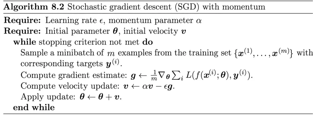
$\alpha$ Typical values are 0.5, 0.9, or 0.99. Usually it starts at a low value that is then raised with time

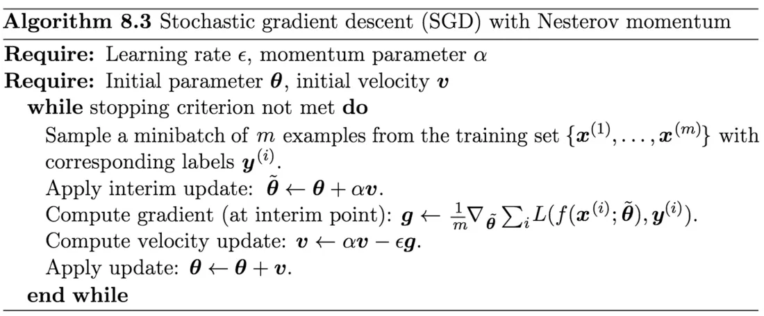
Nesterov momentum:

Just like standard momentum, but use the future gradient (which results in better convergence)

AdaGrad:

Accumulate the global sum of squared gradients for each parameter, and normalize learning rates to achieve fully adaptive updates.

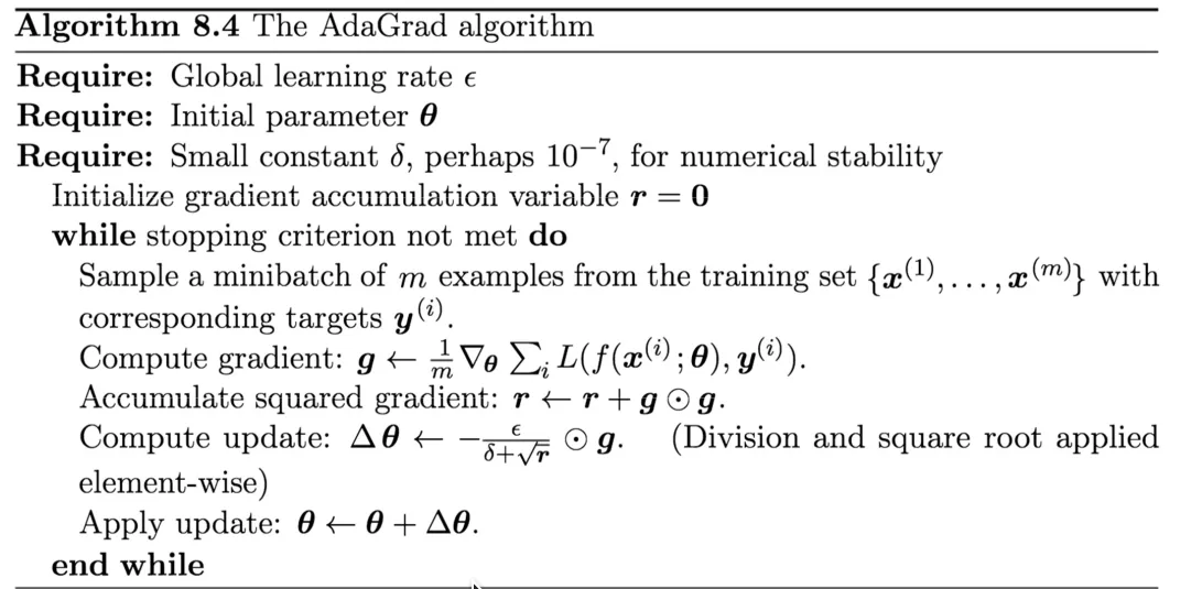
But long history of gradients can slow things down

RMSprop

Replace global accumulation with exponential moving average of squared gradients. Only track recent gradient information to fix the over-decay issue of Adagrad.

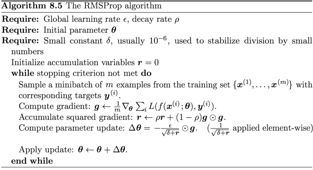
While AdaGrad is designed to work well for convex functions, RMSprop works better in non-convex settings

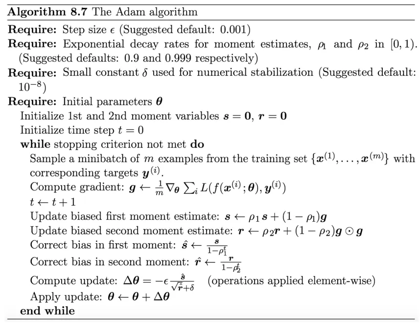
Adam

combining RMSprop with SGD + momentum

Summary：

1st-order information: Gradient $g=∇L(w)$ , describes the slope of the loss landscape.
2nd-order information: Gradient squared / Hessian-related terms, reflects the curvature of the loss landscape.

Optimizer	1st / 2nd Order	Uses historical gradient	Key Features
Momentum	1st-order only	Yes (exponential moving average)	Accelerate convergence, reduce oscillation
Nesterov Momentum (NAG)	1st-order only	Yes (look-ahead + moving average)	More accurate update than standard Momentum
Adagrad	1st + 2nd-order	Yes (cumulative sum of squared gradients)	Per-parameter adaptive lr; learning rate decays continuously
RMSprop	1st + 2nd-order	Yes (moving average of recent squared gradients)	Fix Adagrad’s excessive learning rate decay
Adam	1st + 2nd-order	Yes (EMA for both gradient and squared gradient)	Combine momentum & adaptive lr; robust for most tasks

optimal optimiser:

reading:

优化器可视化 ↗

优化器 ↗

Intro to optimization in deep learning: Momentum, RMSProp and Adam ↗

Regularisation

Deep networks have too many paramerters, lead to overfitting. Possible methods include L1 regularisation, L2regularisation, and Dropout. The goal is to reduce the model capacity

Dataset augmentation

generate transformed version fo input data, suitable for object recognition tasks

Early stopping

stop training when validation set error starts increasing, even if training error is still decreasing

Dropout

Faster training, Less overfitting, Units become more robust

During training, Dropout essentially trains a different sub-network for each batch. At test time, it performs ensemble inference over all these sub-networks. Ensemble learning is a powerful technique to improve generalization performance.

CNN & RNN#

CNN#

Convolution in CNN naturally leverages local information and weight sharing, and achieves translation invariance.

Growing receptive fields（感受野）, Parameter sharing, Convolution with stride

dimention after convolution：

[C, H, W] \times N \cdot [C, H, W] \rightarrow [N \cdot C, \frac{h_{in} - h_{f}}s + 1, \frac{w_{in} - w_{f}}s + 1]

pooling :

downsample, reduces feature map size, cuts computation cost, enlarges receptive fields, retains key features, improves translation invariance and robustness, and mitigates overfitting.

Strided convolution can replace pooling. The core difference is that strided convolution has learnable parameters while pooling does not, and they apply to different scenarios.

history of CNN: Lenet -> Alexnet -> VGG16 -> GoogLeNet -> Inception network V3 -> Resnet

AlexNet:

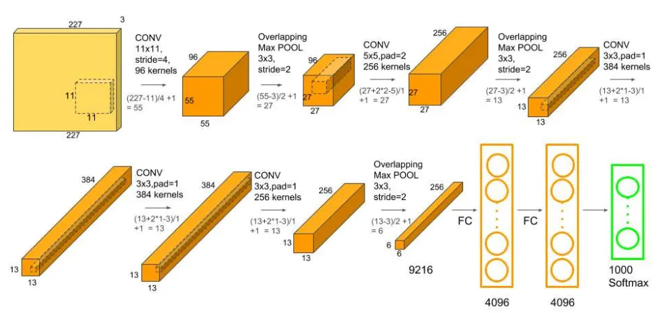
Increasing the number of channels enhances the model’s representational power, allowing it to build complex features from simple ones. Random initialization and data-driven learning make each channel specialize in different patterns, forming complementary detectors that encode full image information.

VGG16:

The number of filters increases with depth.
It uses stacked 3×3 convolutions (2 or 3 in a group).
Stacking small filters achieves the same receptive field as a larger filter (e.g., 2×3×3 = 1×5×5).

More ReLU operations → stronger non-linearity → more powerful model.
Fewer parameters (e.g., 3×3×3=27 vs. 7×7=49), which reduces computation and overfitting risk

GoggleNet

Key features: inception units, batch normalization, image distortions(augmentation), RMSprop key solution to:

Very deep networks are prone to overfitting due to the large number of parameters
Naively stacking large convolution operations is computationally expensive: if two convolutional layers are chained, any uniform increase in the number of their filters results in a quadratic increase of computation make network wider instead of deeper having filters of multiple sizes operating at the same level (Use padding to make sure filter outputs have same size.) 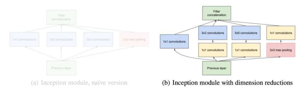This naive version of the Inception unit is very expensive! use 1x1 convolutions to limit the number of channels

The wide multi-branch architecture fuses multi-scale features for stronger feature representation.
1×1 convolutions serve as bottlenecks to reduce computation. Global average pooling removes heavy fully connected layers, making the deep network lightweight.

ResNet

The residual module Introduce skip or shortcut connections Make it easy for network layers to represent the identity mapping

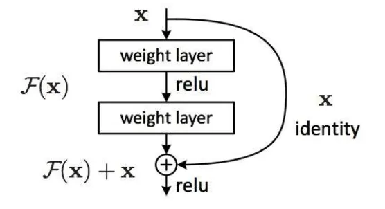
Interpreting ResNets: ResNet has multiple paths with different lengths due to skip connections. Short paths dominate training because they effectively avoid gradient vanishing.

FractalNet

good performance relies on the coexistence of shallow and deep paths, rather than residual connections.

Stochastic depth

randomly drops entire residual blocks during training, while all blocks are active at inference. It creates short paths to avoid gradient vanishing, reduces training cost, and improves generalization by training an ensemble of sub-networks with different depths

Use a trained network for a new task

Treat activations from fully connected layers as fixed features, and only train a new classifier.
Fine-tune the entire network together with the new classifier for better adaptation.

Summary

CNN use convolutions to exploit grid structure
Parameters sharing and sparse connections allow toscale to larger inputs
Pooling introduces invariance to transformations
Modern architectures use several tricks to increase depth and reduce computational cost

Recurrent Neural Networks (RNN)#

Modeling the temporal dependences.Transition matrix: $f(S_t) = f(S_{t-1},X_t)$ if we have $X_t$

Input representation

one-hot
embedding

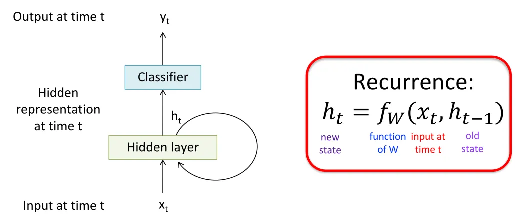
Vanilla RNN Cell:

h_t = \tanh\left( W \begin{pmatrix} x_t \\ h_{t-1} \end{pmatrix} + b \right) = \tanh(W_xx_t + W_hh_{t-1})

\frac{d}{da}\tanh(a) = 1 - \tanh^2(a)

Tanh is zero-centered with a wider useful gradient range. It stabilizes hidden states and eases gradient vanishing in RNNs.

BPTT

The weight updates are computed for each copy in the unfolded network, then summed (or averaged) and applied to the RNN weights
In practice, truncated BPTT is used: run the RNN forward k1 time steps, propagate backward for k2 time steps 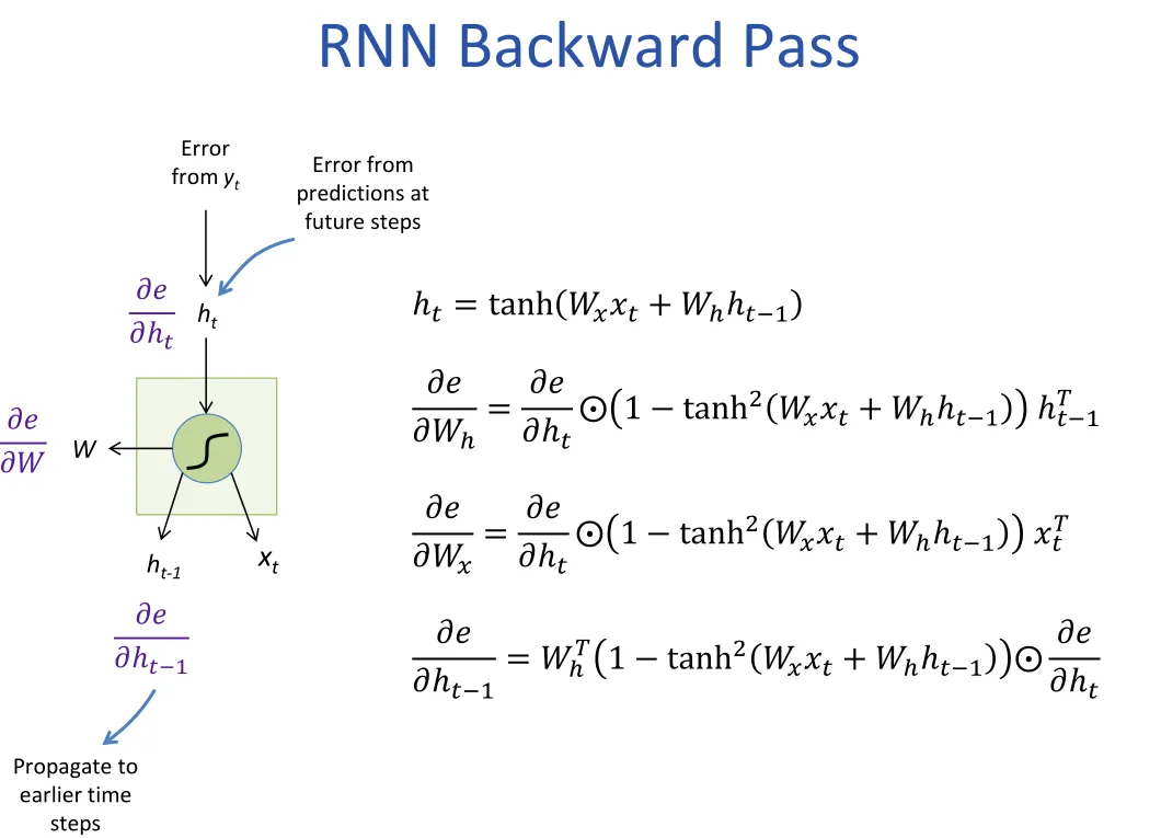For long sequences, this is a problem Vanishing/exploding gradients (Gradients will vanish if largest singular value of $W_h$ is less than 1)

LSTM & GRU

Both are gated RNN variants using gates to control information flow, solve long-term dependency and gradient vanishing problems.

LSTM

Has 3 gates and a long-term memory called cell state Ct.

Forget gate: decide what old info to drop
Input gate: decide what new info to store
Output gate: decide what to output to hidden state

f_t = \sigma(W_f [h_{t-1}, x_t] + b_f)

i_t = \sigma(W_i [h_{t-1}, x_t] + b_i)

o_t = \sigma(W_o [h_{t-1}, x_t] + b_o)

\tilde{C}_t = \tanh(W_C [h_{t-1}, x_t] + b_C)

C_t = f_t \odot C_{t-1} + i_t \odot \tilde{C}_t

h_t = o_t \odot \tanh(C_t)

GRU

Simplified LSTM with 2 gates only, no separate cell state. Faster to train.

Reset gate: control how much past info to forget
Update gate: control how much old state to keep & new info to add

% Gates r_t = \sigma(W_r [h_{t-1}, x_t] + b_r)

z_t = \sigma(W_z [h_{t-1}, x_t] + b_z)

% Candidate hidden state \tilde{h}_t = \tanh(W_h [r_t \odot h_{t-1}, x_t] + b_h)

h_t = (1-z_t) \odot h_{t-1} + z_t \odot \tilde{h}_t

attention & transforemer#

attention is not first intro from transformer Two pain points: long-range dependency problem and lack of parallelism.Transformer uses self-attention and parallel computation to fix them, plus positional encoding for order.

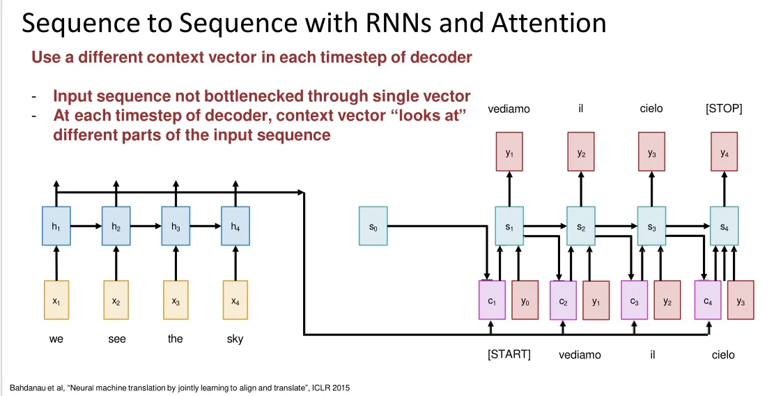
Sequence to Sequence with RNNs : Encoder - Decoder 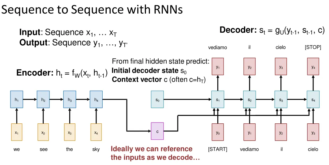During Training: Often, we use the “correct” token state even if the model is wrong. Called teacher forcing During Test-time: from the model’s outputs until we sample [STOP]

Input sequence bottlenecked through fixed-sized vector. What if T=1000? 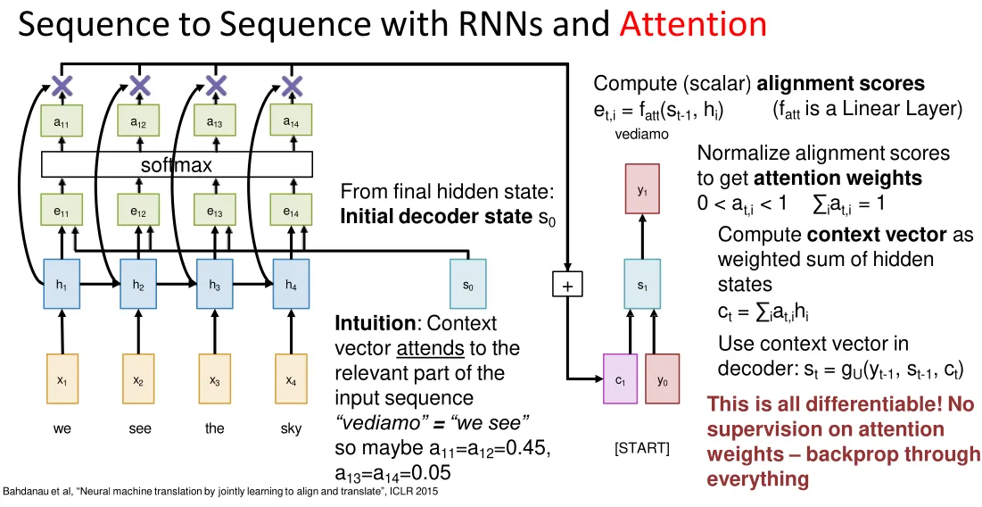Repeat: Use s1 to compute new context vector c2 Compute (scalar) alignment scores $e_{t,i} = f_{att}(s_{t-1}, h_i)$ ( $f_{att}$ is a Linear Layer)

Attention RNN for image captining：

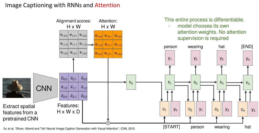Each timestep of decoder uses a different context vector that looks at different parts of the input image

General attention layer

attention operation is permutation invariant.
Change fatt(.) (the function to get alignment) to a dot product, this actually can work well in practice: Dot product increases logit variance, causing softmax to become too sharp. Dividing by D stabilizes the distribution, similar to Xavier/Kaiming initialization.
Multiple query vectors: each query creates a new, corresponding output context vector (Allows us to compute multiple attention context vectors at once)
input vectors are used for both the alignment as well as the attention calculations. (We can add more expressivity to the layer by adding a different FC layer before each of the two steps.)

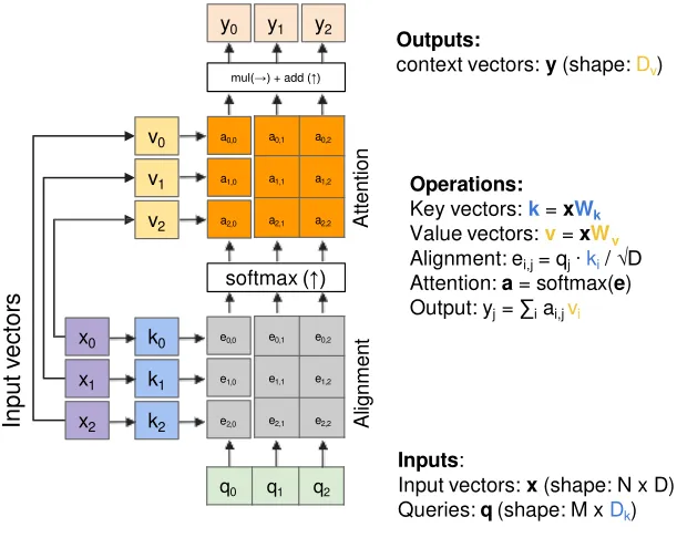
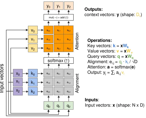
Self-attention leverages the strengths of attention layers without the need for separate query vectors.

[x_0,x_1,x_2]\rightarrow[self-attention]\rightarrow[y_0,y_1,y_2]

Positional encoding

The attention block in the transformer is invariant to the permutation of Key/Values for a give query. Positional embedding: a function mapping positions (of words) into vectors

It should output a unique encoding for each time-step (word’s position in a sentence)
Distance between any two time-steps should be consistent across sentences with different lengths.
The model should generalize to longer sentences without any efforts. Its values should be bounded.
It must be deterministic.

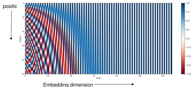
\overrightarrow{p}_t^{(i)} = f(t)^{(i)} := \begin{cases}\sin(\omega_k \cdot t), & \text{if } i = 2k \\ \cos(\omega_k \cdot t), & \text{if } i = 2k + 1\end{cases}, \text{ where }\omega_k = \dfrac{1}{10000^{2k/d}}

Frequencies decreasing along depth for the give position. This is consistent with the trend in the positional binary coding.
It allows the model to attend relative positions effortlessly. since for any fixed offset k, PEpos+k can be represented as a linear function of PEpos

details and proof ↗

We can Add the positional embedding to the token embedding, requires the same number of the dimensions; or Concatenate the positional embedding to the token embedding, dimensions can be different, however, require more memory spaces

positional encoding could also be learnable (but it is difficult to handling squences longer than that seen in training.)

some other positional encoding: Relative positional encodings for text (by Shaw et al 2018) and for image (Bello etal 2019). Complex-value encodings (wang et al 2019). Rotary encodings in Roformer (Su et al 2021) Conditional positional encoding ( Chu et al, ICLR2023).

Masked self-attention layer

A self-attention module with masks to block future positions, ensuring each token only attends to preceding elements, widely used in sequence generation. Allows us to parallelize attention across time

Multi-head self-attention layer

Splits attention into multiple parallel heads to capture diverse types of contextual relationships and enrich feature representation.

Transformer

combine all of above together 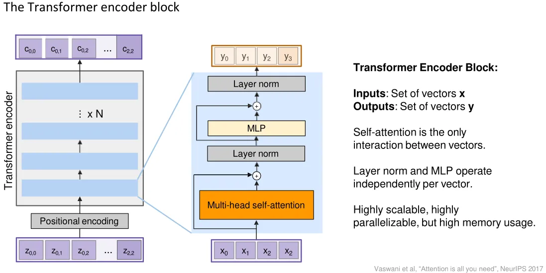Layer Normalization:It normalizes values across feature dimensions of each token, keeping distribution stable and preventing gradients from becoming too small during backpropagation. there could be more MLP (parallel) after LN

Transformers are a type of layer that uses self-attention and layer norm.

It is highly scalable (could parallelize) and highly parallelizable
Faster training, larger models, better performance across vision and language tasks
They are quickly replacing RNNs, LSTMs, and may(?) even replace convolutions.

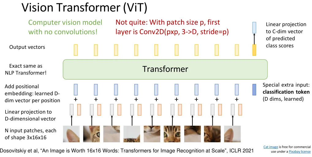
Vision Transformers (ViT)#

Add attention to existing CNNs did not replace convolution entirely
Replace Convolution with “Local Attention”: Lots of tricky details, hard to implement, only marginally better than ResNets
Standard Transformer on Pixels: Memory intensive

VIT: Standard Transformer on Patches

Improving ViT

Regularization for ViT models:

Weight Decay: $L = L_{\text{task}} + \frac{\lambda}{2}\sum w^2 \text{, and }w_{t+1} = w_t - \eta\left( \frac{\partial L_{\text{task}}}{\partial w_t} + \lambda w_t \right)$
Stochastic Depth: $H_{\ell} = \operatorname{ReLU}\big(b_{\ell} \cdot f_{\ell}(H_{\ell-1}) + H_{\ell-1}\big),\ b_{\ell} \in \{0,1\}$
Dropout (in FFN layers of Transformer)

Data Augmentation for ViT models:

MixUp: Linearly interpolates pairs of samples and labels to regularize model.
RandAugment: Applies random combinations of basic image augmentations with limited magnitude.

Distillation: Train a teacher model on images and ground-truth labels Train a student model to match predictions from the teacher (sometimes also to match GT labels) (Add a distillation woken as Classification token, to predict class scores; should match teacher)

Hierarchical ViT: Swin Transformer

Standard ViT uses an isotropic design with fixed resolution and channels, which lacks the multi-scale hierarchical feature extraction of CNNs. Thus researchers propose hierarchical ViT to introduce resolution downsampling and channel expansion, just like CNNs, to better handle multi-scale objects in images.

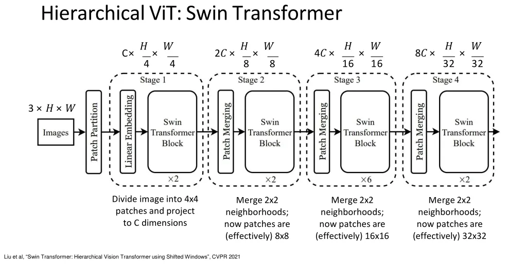
Window attention & Shifted window attention ↗

don’t use full attention, instead use attention over patches tokens only interact with other tokens within the same window; no communication across windows -> Shifted Window Attention

\operatorname{SW-Attention}(Q,K,V) = \operatorname{Softmax}\left(\frac{QK^\top}{\sqrt{d}}+B+M\right)V

teacher’s takeaway

Vison transformers are an evolution, not a revolution. Main benefit is probably speed

Self-Supervised Learning#

Model is trained to predict some naturally-occurring signal in the raw data rather than human annotations. Model learn some underlying hidden structure of the data

Pretrain a network on a pretext task that doesn’t require supervision, and Transfer encoder to downstream tasks via linear classifiers, KNN, finetuning. Goal: Pretrain + Transfer does better than supervised pretraining, and better than directly training on downstream

Generative: Predict missing input content AutoEncoder (sparse/denoising/masked), Autoregressive, GANs, Colorization, Inpainting
Discriminative: Predict input attributes Context prediction, Rotation, Clustering, Contrastive learning
Multimodal: Combine RGB with other signals Video, 3D, Sound, Language

Autoencoders are data-dependent, lossy in reconstruction, and can learn representations automatically from training samples.

Autoencoder tries to reconstruct inputs. Hidden layer (hopefully) learns good representations H < D is the only thing forcing non-trivial hidden representations

sparse AE

(H > D)Sparse autoencoders map inputs to a high-dimensional hidden layer and apply sparsity constraints. The constraints keep the average activation of most neurons low, so only a small number of neurons are activated to learn meaningful features.

Many ways to implement sparsity penalties. Sparse activation means only a few neurons fire. Such features correspond to distinct visual patterns, thus being more interpretable.

Denoising AE

reconstruct the clean version of the noisy inputs

VAE (variational AE): Next part

Context Prediction 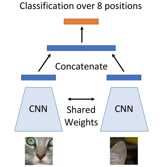Two networks with shared weights sometimes called a ”Siamese network”

Extension: Solving Jigsaw Puzzles The image is split into 9 patches and shuffled. The model takes these patches as input and predicts their correct permutation via fully connected layers.

Context Encoders Learning by Inpainting: Input -> Encoder -> Decoder -> output

Colorization

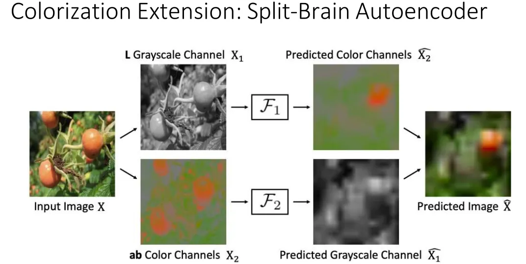Generative pretext tasks force the model to learn trivial pixel-level details (e.g., precise color tones) that are useless for downstream tasks. Split-Brain Autoencoder solves this by predicting one set of image channels from another, focusing on meaningful cross-channel relations instead of exact pixel reconstruction.

Deep Clustering

Deep Clustering jointly learns data representations and cluster assignments via neural networks. It uses an autoencoder to compress input into low-dimensional features, then iteratively clusters features (e.g., K-means) and trains the network with cluster-based loss, grouping similar samples without labels.

It is hard to fairly compare SSL methods due to diverse experimental settings, including network architectures, datasets, evaluation protocols and hyperparameters.

Contrastive representation learning#

awesome blog ↗

SimCLR, MOCO, MAE, CLIP(modality contrastive learning)

pretext tasks are built on image transformations, yet their learned representations are task-specific. Researchers aim to design more general pretext tasks for better feature transfer.

Formulation:

score(f(x),f(x^+))>>score(f(x),f(x^-))

we aim to learn an encoder function f that yields high score for positive pairs $(x, x^+)$ and low scores for negative pairs $(x, x^-)$ .

InfoNCE loss

L_{InfoNCE}=−E_x[log\frac{exp(f(x,y))}{exp(f(x,y))+∑_{i=1}^{N−1}exp(f(x,yi))}]

Looks like Cross entropy loss for a N-way softmax classifier!

-\sum_{x} p(x)\log q(x)

p(x): Ground-truth distribution, represented as one-hot encoding.

q(x): Model prediction distribution obtained via softmax.

Minimizing the InfoNCE loss is equivalent to maximizing the lower bound of mutual information between two variables.

proof ↗

I(X;Y)≥log(N)−L_{InfoNCE}

The larger the negative sample size (N), the tighter the bound

Variational Bounds on Mutual Information ↗

Mathematical Foundations of Contrastive Loss ↗

SimCLR

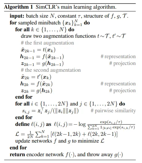
Projection head: Linear or non-linear projection heads boost representation learning. The contrastive loss may drop useful features; the head keeps more information in the encoder output space.
Large batch size: Large batches are essential for SimCLR, but bring high memory cost, requiring distributed training with TPUs.
For any sample in a batch of 2N augmented views, there is only 1 positive pair and 2N−2 negatives.
Drawbacks: extreme positive-negative imbalance, heavily relies on large batch size and high computing resources.

MOCO

Momentum Contrastive Learning

Keep a running queue of keys (negative samples).
Compute gradients and update the encoder only through the queries. (The key encoder disables gradient computation to maintain stable negative samples in the queue and ensure steady training.)
Decouple min-batch size with the number of keys: can support a large number of negative samples.
The key encoder is slowly progressing through the momentum update rules:

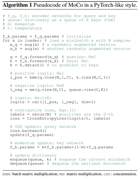
\theta_k\leftarrow m\theta_k+(1-m)\theta_q

MOCO V2

combine SimCLR & MoCo

From SimCLR: non-linear projection head and strong data augmentation.
From MoCo: momentum-updated queues that allow training on a large number of negative samples (no TPU required!).

MAE

A old method dethrones contrastive learning. Denoising Autoencoder with Vision Transformer

input (full image) → patch embedding → shuffle & mask (keep 25%) → Encoder (ViT) (only visible patches) → concat mask tokens → unshuffle (restore original order) → add full positional embedding → Decoder (light ViT) → output (reconstruct image) → MSE loss on masked patches

Multimodal Self-Supervised Learning

Video, Sound, 3D, Language

Language：

Semantic density: Just a few words give rich information
Universality: Language can describe any concept
Scalability: Non-experts can easily caption images; data can also be collected from the web at scale

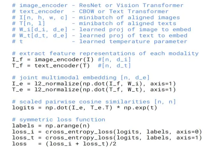
CLIP

${v_i}$ : Image feature vector of the i-th image
${t_j}$ : Text feature vector of the j-th text
$L_{I→T}$ : Loop over every row (each image), treat all texts in the batch as candidates.
$L_{T→I}$ : Loop over every column (each text), treat all images in the batch as candidates.

S_{ij} = v_i \cdot t_j

\mathcal{L}_{\text{InfoNCE}} = -\frac{1}{N}\sum_{i=1}^N \log\frac{e^{S_{ii}/\tau}}{\sum_{j=1}^N e^{S_{ij}/\tau}}

\mathcal{L} = \mathcal{L}_{I \to T} + \mathcal{L}_{T \to I}

\min \mathcal{L}_{\text{InfoNCE}} \iff \max \; \text{lower bound of } I(v;t)

VAE & GAN#

VAE#

We can use autoencoders for data generation via latent code z. However, standard autoencoders do not regularize the distribution of z, so we cannot easily sample valid latent codes.

Instead of outputting a single latent vector, VAE produces a Gaussian distribution $N(\mu,\sigma)$ . It models the latent distribution for each input $x$ . Then, we can sample a representation/code $z$ from $q_θ(z∣x)$ (where the subscript θ means that the probability is parametrised by θ), the decoder is another NN like $p_ϕ(x∣z)$

Loss

loss function for i-th datapoint - the total loss is the sum of all the $l_i$

$\log p_ϕ(x∣z)$ measure the information loss from low demention z to high demention x, This term encourages decoder to learn to reconstruct the data.
KL divergence is regularisation term - measures how close q is to p, This make sure the encoder doesn’t cheat and map each datapoint in different regions of the space

l_i(\theta, \phi) = -\mathbb{E}_{z \sim q_\theta(z|x_i)}\left[\log p_\phi(x_i|z)\right] + KL\left(q_\theta(z|x_i) \parallel p(z)\right)

The prior distribution of latent variables $p(z)$ is set to standard Gaussian distribution $\mathcal{N}(0,1)$ . The model regularizes the encoded distribution to approach the prior, forming a continuous and smooth latent space for new sample generation.

KL divergence ↗

variational

In this context, learning is called inference

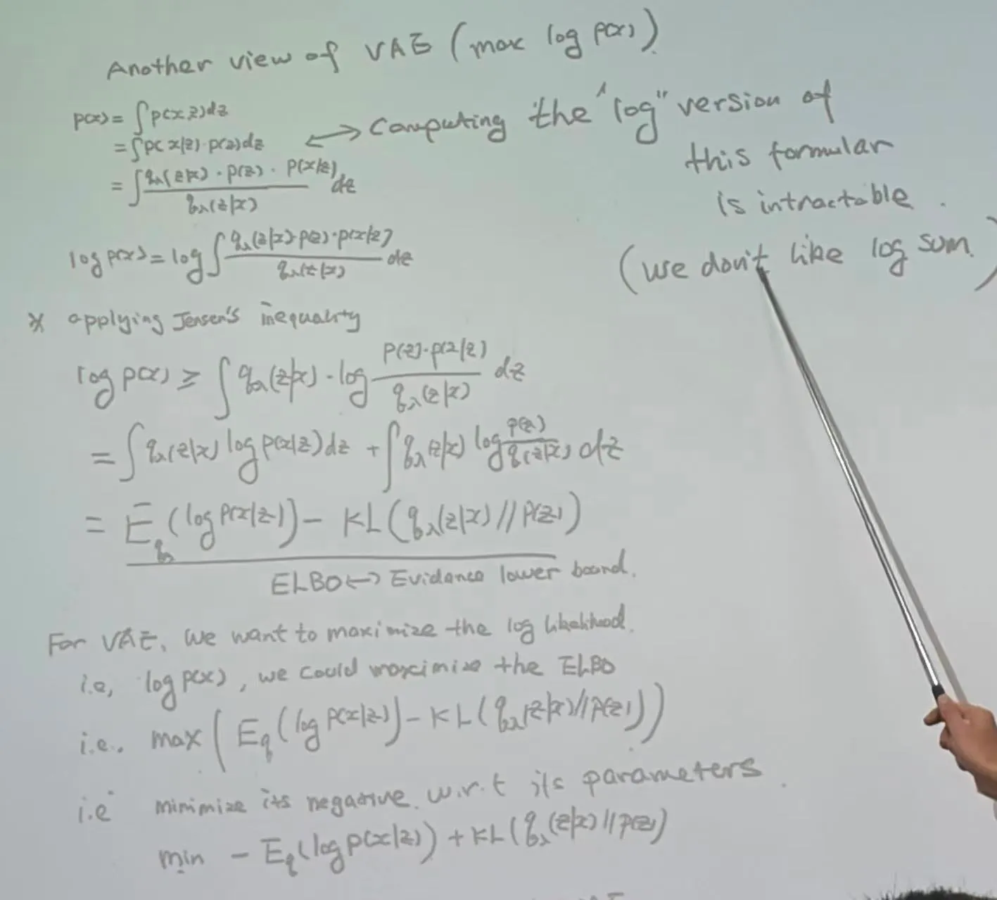
Variational inference is an approximate method in probabilistic machine learning. The true posterior distribution $p(z∣x)$ is intractable due to high-dimensional integration ( $p(x)=∫p(x∣z)p(z)dz$ ).

Objective: maximize $\log p(x)$

probabilistic perspective

we use a simple, parameterized distribution $q_\lambda(z∣x)$ to approximate $p(z∣x)$ . Minimize the KL divergence $\mathrm{KL}\big(q_\lambda(z\mid x) \parallel p(z\mid x)\big)$ to perform variational inference, which leads to the ELBO objective.

\mathrm{KL}\big(q_\theta(z\mid x) \parallel p(z\mid x)\big) = \mathbb{E}_{q_\theta(z\mid x)}\left[\log\frac{q_\theta(z\mid x)}{p(z\mid x)}\right]

Substitute Bayes’ rule

p(z\mid x) = \dfrac{p(x\mid z)p(z)}{p(x)}

\mathrm{KL}\big(q_\theta(z\mid x) \parallel p(z\mid x)\big) = \mathbb{E}_{q_\theta(z\mid x)}\big[\log q_\theta(z\mid x)\big] - \mathbb{E}_{q_\theta(z\mid x)}\big[\log p(x\mid z)\big] - \mathbb{E}_{q_\theta(z\mid x)}\big[\log p(z)\big] + \log p(x)

Rearrange to get ELBO

\log p(x) = \underbrace{\mathbb{E}_{q_\theta(z\mid x)}\big[\log p(x\mid z)\big] - \mathrm{KL}\big(q_\theta(z\mid x) \parallel p(z)\big)}_{\text{ELBO}} + \mathrm{KL}\big(q_\theta(z\mid x) \parallel p(z\mid x)\big)

Optimization target: minimize KL $\iff$ maximize ELBO Final loss (negative ELBO):

\mathcal{L}(\theta,\phi) = -\mathbb{E}_{z\sim q_\theta(z\mid x)}\big[\log p_\phi(x\mid z)\big] + \mathrm{KL}\big(q_\theta(z\mid x) \parallel p(z)\big)

Maximising ELBO means 1) q close to p and 2) higher p (better generator)

Generative / Reconstruction Perspective

We maximize the evidence lower bound to indirectly optimize the log-likelihood of observed data.

prof. jianguo’s scripts

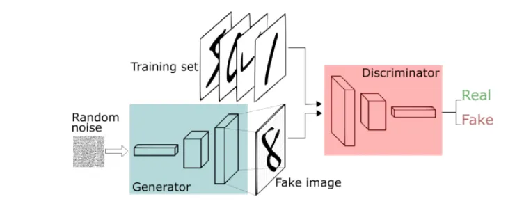
GAN#

Generative adversarial networks: can we learn just the generator?

GANs propose to learn the loss function
The training process is a game between two networks
Generator: learns to generate samples
Discriminator: learns to distinguish between generated and real samples
Adversarial training: the generator tries to fool the discriminator while the discriminator tries to get better at distinguishing fake vs real images. When the discriminator spots a fake the generator adjusts its parameters, until at the end the generator reproduces the true data distribution and the discriminator is unable to find differences Note: both the generator and the discriminator need to be differentiable minimax strategy

\min_{G} \max_{D} V(D,G) = \mathbb{E}_{x \sim p_{\text{data}}} \big[\log D(x)\big] + \mathbb{E}_{z \sim p_z} \big[\log\big(1-D(G(z))\big)\big]

Symbol	Meaning
$D$	Discriminator network, outputs a value in [0,1]: probability that the input is real data
$G$	Generator network, maps random noise z to fake samples
$p_{data}$	Distribution of real training data
$p_z$	Prior distribution of latent noise (usually standard Gaussian)
$E[⋅]$	Expectation, calculates the average value over sampled data

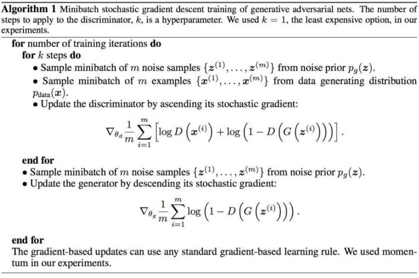
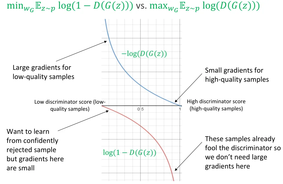
Gradient ascent for discriminator to tell real and fake samples apart.

D^* = \arg\max_D V(G,D)

Theoretical gradient descent for generator to fool discriminator.

G^* = \arg\min_G \mathbb{E}_{z\sim p_z}\big[\log(1-D(G(z)))\big]

Practical gradient ascent to avoid gradient vanishing.

G^* = \arg\max_G \mathbb{E}_{z\sim p_z}\big[\log D(G(z))\big]

Problems

Finite sample size: training set is finite, not the full distribution
Limited capacity: the generator has limit capacity, i.e. cannot perfectly represent any distribution
Optimisation errors: optimisers can get stuck in local optima or never exactly converge to global optima
Saddle point problem: harder than finding a maximum or minimum
Balancing updates: D too weak/strong means no gradient for G to improve

CGAN (conditioanl GAN)

G(z,c),\ D(x,c)

Both generator and discriminator take an additional condition embedding $c$ to perform conditional generation.

The GAN objective is conditioned on $c$ , guiding the model to generate samples matching the given condition.

diffusion model#

Awsome blog ↗(Weng, Lilian. (Jul 2021). What are diffusion models? Lil’Log.)

A good blog ↗

Idea: Estimating and analyzing small step sizes is more tractable/easier than a single step from random noise to the learned distribution.
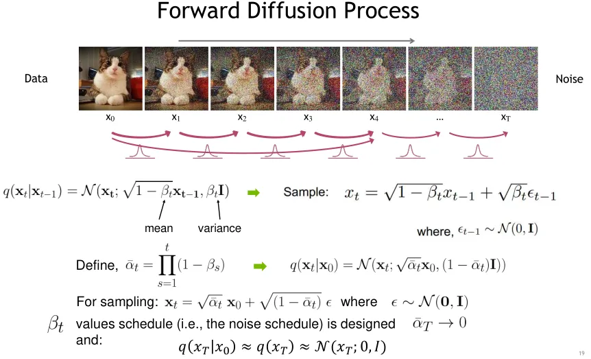
Convert a well-known and simple base distribution (like a Gaussian) to the target (data) distribution iteratively, with small step sizes, via a Markov chain:
Denoising diffusion models consist of two processes:
- Forward diffusion process that gradually adds noise to input

q(\mathbf{x}_t) = \int q(\mathbf{x}_0) q(\mathbf{x}_t|\mathbf{x}_0) d\mathbf{x}_0

we can Sample clean data:

\mathbf{x}_0 \sim q(\mathbf{x}_0)

, then sample diffused data:

\mathbf{x}_t \sim q(\mathbf{x}_t|\mathbf{x}_0) = \sqrt{\bar{\alpha}_t}\mathbf{x}_0 + \sqrt{1-\bar{\alpha}_t}\epsilon

Reverse denoising process that learns to generate data by denoising Generative Learning by Denoising: At $t=T$ , the distribution becomes pure noise:

q(\mathbf{x}_T) \approx \mathcal{N}(\mathbf{x}_T; \mathbf{0}, \mathbf{I})

We can sample noise:

\mathbf{x}_T \sim \mathcal{N}(\mathbf{0}, \mathbf{I})

then Iteratively denoise:

\mathbf{x}_{t-1} \sim q(\mathbf{x}_{t-1}|\mathbf{x}_t)

Since $q(\mathbf{x}_{t-1}|\mathbf{x}_t)$ is unknown, we approximate it with a normal distribution (valid when ${\beta_t \in (0,1)}_{t=1}^T$ is small). so

p_\theta(\mathbf{x}_{t-1} \mid \mathbf{x}_t) = \mathcal{N}\big(\mathbf{x}_{t-1}; \boldsymbol{\mu}_\theta(\mathbf{x}_t, t), \boldsymbol{\Sigma}_\theta(\mathbf{x}_t, t)\big)

In practice, $Σ$ is set to $\sigma_t^2I$ ( $\sigma_t$ as hyperparameter), so we only need to learn the mean of the distribution

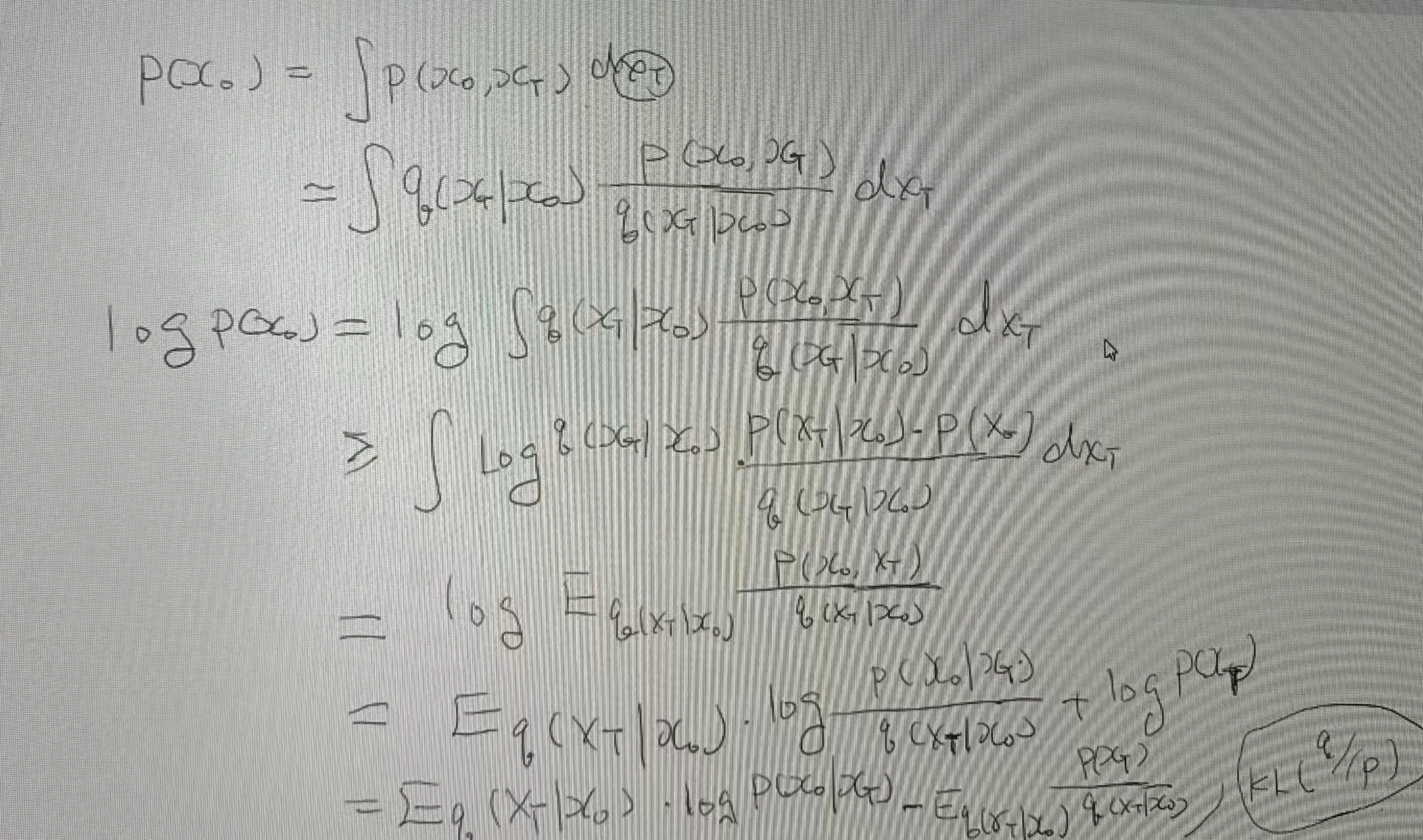
Training a Diffusion Model

Objective: learn $p_\theta(\mathbf{x}_{t-1} \mid \mathbf{x}_t)$ , more precisely $\boldsymbol{\mu}_\theta(\mathbf{x}_t, t)$ (by U-net)

GT (Posterior Distribution): $q(\mathbf{x}_{t-1} \mid \mathbf{x}_t,\mathbf{x}_0) = \mathcal{N}\big(x_{t-1}; \hat{\boldsymbol{\mu}}_t(x_t, x_0), \hat{\beta}_t \mathbf{I}\big)$ , where $\tilde{\mu}_t(x_t, x_0) = \frac{\sqrt{\alpha_t}(1-\bar{\alpha}_{t-1})x_t + \sqrt{\bar{\alpha}_{t-1}}\beta_t x_0}{1-\bar{\alpha}_t}$ and $\tilde{\beta}_t = \frac{1-\bar{\alpha}_{t-1}}{1-\bar{\alpha}_t}\beta_t$ , In the reverse process, the transition cannot be factorized into a simple single-step dependency: 为什么反向markov不能只看一步？.

by bayesian

q(x_{t-1} \mid x_t, x_0) = \frac{q(x_t \mid x_{t-1}) \, q(x_{t-1} \mid x_0)}{q(x_t \mid x_0)}

q(x_t \mid x_{t-1}) = \mathcal{N}(x_t; \sqrt{\alpha_t}x_{t-1}, \beta_t I), \quad \alpha_t = 1-\beta_t

q(x_t \mid x_0) = \mathcal{N}(x_t; \sqrt{\bar{\alpha}_t}x_0, (1-\bar{\alpha}_t)I), \quad \bar{\alpha}_t = \prod_{i=1}^t \alpha_i

Loss (KL divergence, ELBO) or simply align $\mu_\theta \ \& \ \tilde{\mu}_t \text{ with MSE}$ (this two is equivalent for $L_{t-1}$ ):

\mathbb{E}_q\left[ \underbrace{D_{\text{KL}}\big(q(x_T|x_0) \parallel p(x_T)\big)}_{L_T} + \sum_{t>1} \underbrace{D_{\text{KL}}\big(q(x_{t-1}|x_t,x_0) \parallel p_\theta(x_{t-1}|x_t)\big)}_{L_{t-1}} - \underbrace{\log p_\theta(x_0|x_1)}_{L_0} \right]

L_{t-1} = \mathbb{E}_q\left[ \frac{1}{2\sigma_t^2} \left\| \tilde{\mu}_t(x_t, x_0) - \mu_\theta(x_t, t) \right\|^2 \right] + C

and also, We can get

\tilde{\mu}_t(x_t, x_0) = \frac{\sqrt{\alpha_t}(1-\bar{\alpha}_{t-1})x_t + \sqrt{\bar{\alpha}_{t-1}}\beta_t x_0}{1-\bar{\alpha}_t} = \frac{1}{\sqrt{\alpha_t}}\left(x_t - \frac{\beta_t}{\sqrt{1-\bar{\alpha}_t}}\epsilon\right), \text{becuase } \mathbf{x}_t \sim q(\mathbf{x}_t|\mathbf{x}_0) = \sqrt{\bar{\alpha}_t}\mathbf{x}_0 + \sqrt{1-\bar{\alpha}_t}\epsilon

so we can just predict the residual (the added noise) $\epsilon_\theta(x_t, t)$ (by Unet)

loss

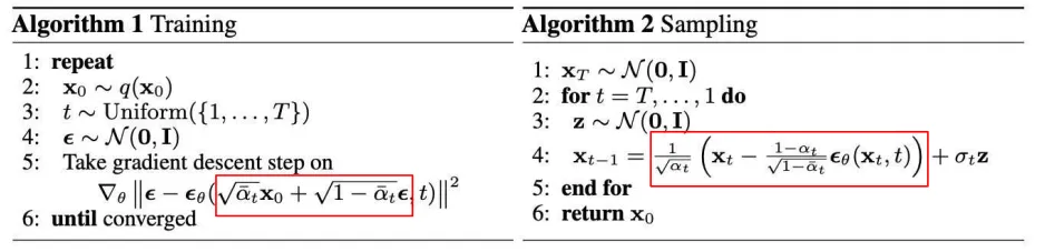
L_{\text{simple}} = \mathbb{E}_{\mathbf{x}_0 \sim q(\mathbf{x}_0), \epsilon \sim \mathcal{N}(\mathbf{0}, \mathbf{I}), t \sim \mathcal{U}(1, T)} \left[ \left\| \epsilon - \epsilon_\theta\left( \underbrace{\sqrt{\bar{\alpha}_t} \mathbf{x}_0 + \sqrt{1-\bar{\alpha}_t} \epsilon }_{\mathbf{x}_t}, t \right) \right\|^2 \right]

But Why we just pridict the niose is OK?

We can prove The noise-prediction objective is mathematically equivalent to optimizing the evidence lower bound (ELBO) of the log-likelihood, under the DDPM’s Gaussian reverse process parameterization with fixed variances.

This is beyond the scope of this course, we can just look through the blog I cited

prof. jianguo’s scripts

Implementation

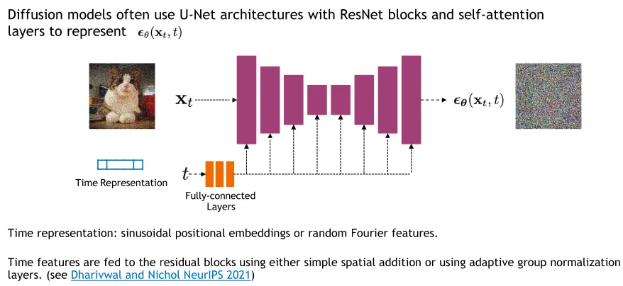
In the forward diffusion, the high frequency content is perturbed faster.
In reverse process: at small t The denoising model is specialized for generating the high-frequency content (i.e., low-level details), and at large t the denoising model is specialized for generating the low-frequency content (i.e., coarse content) So The weighting of the training objective for different timesteps is important!

Conditional diffusion models#

Include condition as input to reverse process The reverse process is modified into a conditional distribution:

p_\theta(\mathbf{x}_{0:T}|\mathbf{c}) = p(\mathbf{x}_T)\prod_{t=1}^T p_\theta(\mathbf{x}_{t-1}|\mathbf{x}_t, \mathbf{c})

At each step:

p_\theta(\mathbf{x}_{t-1}|\mathbf{x}_t, \mathbf{c}) = \mathcal{N}\big(\mathbf{x}_{t-1}; \boldsymbol{\mu}_\theta(\mathbf{x}_t, t, \mathbf{c}), \boldsymbol{\Sigma}_\theta(\mathbf{x}_t, t, \mathbf{c})\big)

The model’s mean $\boldsymbol{\mu}_\theta$ and variance $\boldsymbol{\Sigma}_\theta$ both take the condition c as input.

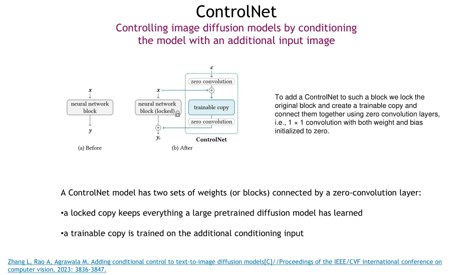
Condition Injection into U-Net - Scalar conditioning (e.g., class labels, style): Encode the scalar into a vector embedding, then inject it via spatial addition or adaptive group normalization (AdaGN).
Image conditioning (e.g., sketches, masks): Concatenate the conditional image with the input image along the channel dimension.
Text conditioning (e.g., prompts): - Single vector embedding: Use spatial addition or AdaGN. - Sequence of vector embeddings (e.g., word tokens): Use cross-attention.

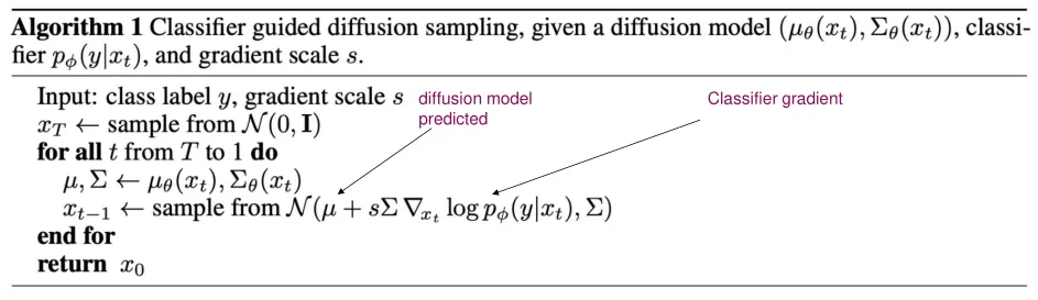
Classifier guidance: a tool for conditional generation

Using the gradient of a trained classifier as guidance

Objective: To optimize the conditional distribution $p(x∣y)$ such that the generated samples x are both realistic and aligned with the condition y.

Denoising process can also be thought as:

Using denoising U-Net to predict gradient
Predicted noise as gradient to update $𝑥_t → 𝑥_{t−1}$
Direction to clean image $∇𝑥_t \log 𝑞(𝑥_t | 𝑥_0)$ (the predicted “score function”)

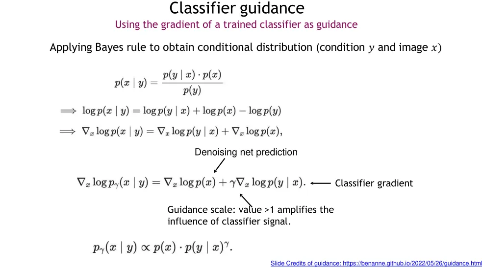
Need to train a separate ”noise-robust” classifier + unconditional diffusion model. Gradient of the classifier w.r.t. input yields arbitrary values

CFG (Classier free guidance) CFG amplifies the difference between conditional and unconditional noise predictions from the same model to strengthen adherence to given conditions. 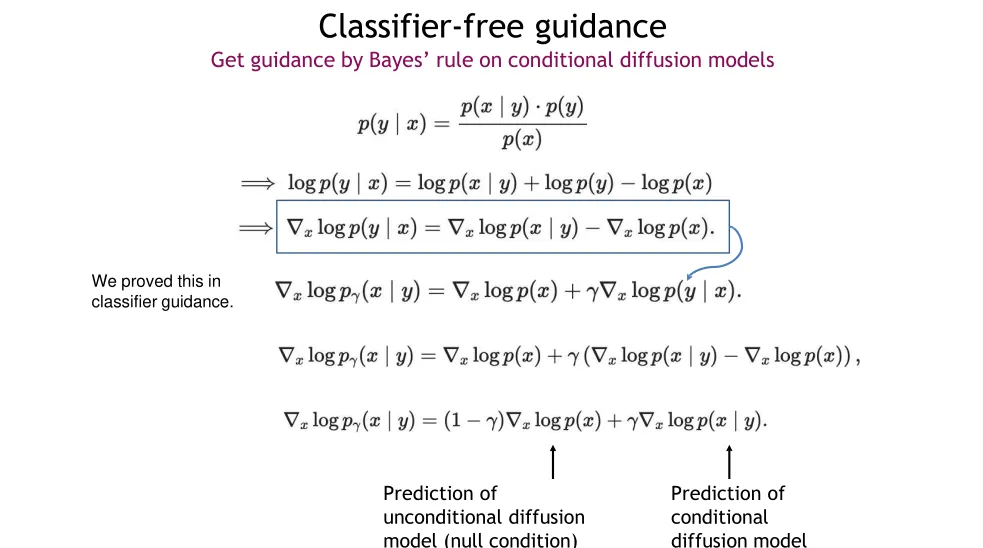Train conditional & unconditional diffusion model jointly via drop-out. All pixels in input receive equally ‘good’ gradients. (CG: Gradients concentrate on local regions only. Pixels get uneven & noisy gradients.)

Some other application

Object Detection#

Predict: bounding boxes, class labels, confidence scores 2 stage -> 1 stage -> other detectors

Two-stage Detectors#

Multiple Objects

Multitask Loss (many things to predict), Each image needs a different number of outputs
Problem: Need to apply CNN to huge number of locations, scales, and aspect ratios, very computationally expensive!

Region Proposals: Selective Search

Intersection over Union (IoU)

for evaluation

\text{IoU} = \frac{\text{Intersection}}{\text{Union}}

Non-maximum suppression (NMS)

Problem: Detectors often output many overlapping detections

Solution: Post-process raw detections using Non-Max Suppression (NMS)

1. Select next highest-scoring box
2. Eliminate lower-scoring boxes with IoU > threshold (e.g. 0.7)
3. If any boxes remain, GOTO 1

txt

Evaluating object detectors

Run object detector on all test images (with NMS)
For each category, compute Average Precision (AP) or area under Precision vs. Recall Curve

\text{𝑃𝑟𝑒𝑐𝑖𝑠𝑖𝑜𝑛} = \frac{\text{t𝑟𝑢𝑒 𝑝𝑜𝑠𝑖t𝑖𝑣𝑒 𝑑𝑒t𝑒𝑐t𝑖𝑜𝑛𝑠}}{\text{t𝑜t𝑎𝑙 𝑑𝑒t𝑒𝑐t𝑖𝑜𝑛𝑠 𝑠𝑜 𝑓𝑎𝑟}}

\text{𝑅𝑒𝑐𝑎𝑙𝑙} = \frac{\text{t𝑟𝑢𝑒 𝑝𝑜𝑠𝑖t𝑖𝑣𝑒 𝑑𝑒t𝑒𝑐t𝑖𝑜𝑛𝑠}}{\text{t𝑟𝑢𝑒 𝑝𝑜𝑠𝑖t𝑖𝑣𝑒 t𝑒𝑠t 𝑖𝑛𝑠t𝑎𝑛𝑐𝑒𝑠}}

For each detection (highest to lowest score) -If it matches some GT box with IoU > 0.5, mark it as positive and eliminate the GT -Otherwise mark it as negative -Plot a point on PR Curve

Two-stage Detectors

R-CNN

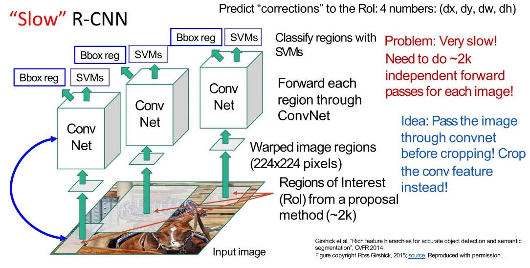
Fast R-CNN

Fast R-CNN still generates proposals on the original image, then uses RoI Pooling and RoI Align to crop corresponding regions from the feature map.

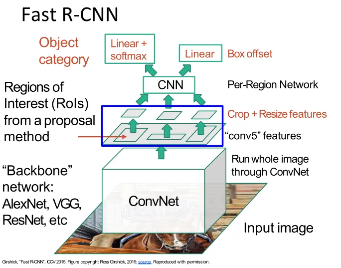
RoI Pooling

First rounding：Align the coordinates of the RoI (from the original image) to integer pixel boundaries on the feature map.
Second rounding：When dividing the mapped RoI into a fixed number of bins, round the boundaries of each bin to integer coordinates.
Apply max pooling to each bin to obtain fixed-size region features.

RoI Align Eliminates rounding errors entirely by using floating-point coordinates and bilinear interpolation to sample values at sub-pixel positions. The bilinear interpolation formula is: $f_{xy} = \sum_{i,j=1}^2 f_{i,j} \max(0, 1 - |x - x_i|) \max(0, 1 - |y - y_j|)$ Then apply max pooling to the sampled values to obtain region features without spatial misalignment.

Faster R-CNN

RPN: The Region Proposal Network (RPN) generates object proposals on the shared feature map output by the CNN. It places multiple (K) multi-scale anchors at each spatial location, performing binary classification (foreground/background) and bounding-box regression to select ~300 high-quality foreground proposals for the subsequent RoI head.

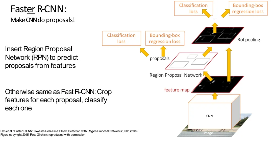
First stage: Run once per image

Backbone network
Region proposal network Second stage: Run once per region
Crop features: RoI pool / align
Predict object class
Prediction bbox offset

Jointly train with 4 losses:

RPN classify object / not object
RPN regress box coordinates
Final classification score (object classes)
Final box coordinates

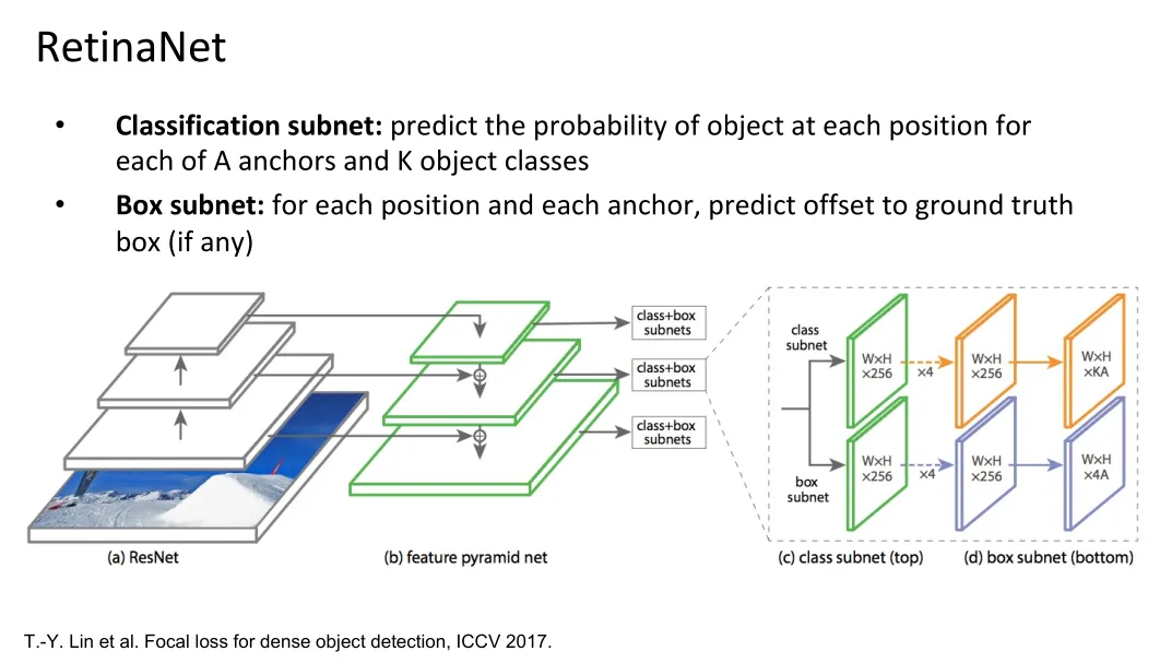
Single-Stage Object Detectors#

put proposal generation and region classification together so that we can do detection in one-shot

Within each grid cell:

Regress from each of the B base boxes to a final box with 5 numbers: $(dx, dy, dh, dw, confidence)$
Predict scores for each of C classes (including background as a class)
Looks a lot like RPN, but category-specific! Output:
7 x 7 x (5 * B + C)

YOLO

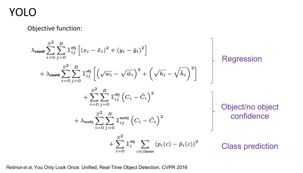
Each grid cell predicts only two boxes and can only have one class – this limits the number of nearby objects that can be predicted

Multi-resolution prediction: SSD

Improve predictive power of lower-level feature maps by adding contextual information from higher-level feature maps
Predict different sizes of bounding boxes from different levels of the pyramid (but share parameters of predictors)

Other Detectors#

transformer based detector

DETR (DEtection TRansformer)

Basic idea:

Extracting features using CNN backbone network;
Learning global features using Transformer encoder;
Generate prediction boxes using Transformer decoder;
Match the prediction box with the ground truth box to calculate the loss;

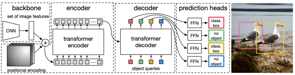
Learning a fixed number of object queries using transformer decoder
Predict one box and class for each query by FNN
Using the Hungarian matching algorithm to match predicted boxes with ground truth boxes and calculate loss. Matched queries are treated as positive samples, while unmatched ones are regarded as negative samples. Positive samples are supervised by classification loss and regression loss to learn to detect objects. Negative samples are only supervised by classification loss (background) to learn to reject background.

Hungarian matching algorithm & KM alg ↗

KM alg ↗

DINO (DETR with Improved deNoising anchOr boxes)

Innovations:

Contrastive denoising training (CDN)

CDN (Contrastive Denoising) is a training-only, plug-and-play module that complements DETR without altering its native pipeline.

In CDN, both positive and negative queries are generated entirely relative to the ground-truth box. Positive queries are created by adding minor geometric offsets to the ground truth to help the model learn precise localization recovery, while negative queries are created by applying larger offsets to the ground truth, forcing the model to learn to reject these nearby distracting boxes as no-object.

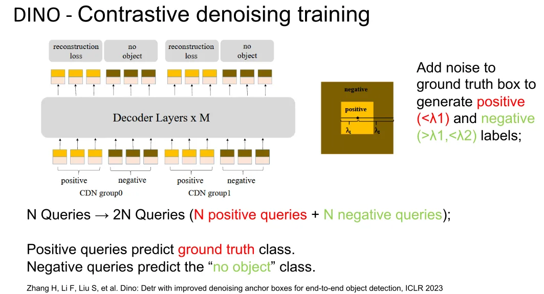
noise refers to the random geometric offsets applied to a ground-truth box to simulate prediction errors, while lambda is the human-defined hyperparameter that scales this noise by setting the maximum allowed ratio of position and size deviation.

During training, for each of the $N$ ground-truth (GT) boxes in an image, CDN generates one positive and one negative sample, feeding a total of $2N$ CDN queries into the decoder. Using a strict attention mask, these $2N$ queries are completely isolated from the native matching queries to enable parallel computation without mutual interference. During inference, the CDN component is fully bypassed, leaving only the native queries. This design keeps the test phase clean and efficient while leveraging the $2N$ contrastive queries during training to significantly enhance the model’s boundary awareness and localization precision.
Mixed query selection
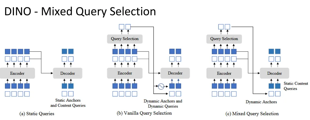
- Static Queries (In DETR) : Decoder queries are static embeddings without taking any encoder features from an individual image. They learn anchors or positional queries from training data and set the content queries as 0 vectors.
- Vanilla Query Selection (In Deformable DETR) : It selects positions with top K classification scores as reference points and the content queries are linear transform of the positional embeddings of the reference points.
- Mixed Query Selection (In DINO) : Using selected positions as anchors and learnable query embeddings as the content queries. (Only enhances location queries with top-K selection features and maintains the learnability of content queries. This helps the model to utilize better positional information to gather more comprehensive content features from the encoder)

Query Type	Positional Query Source (Where)	Content Query Source (What)	Core Philosophy
Static (DETR)	Static, learnable dataset priors	Constant $0$ vectors	Completely blind to the input image at initialization.
Vanilla (Deformable DETR)	Top-K locations from Encoder	Linear transformation of Positional Query	Fully tied to the image; content is strictly bound to position.
Mixed (DINO)	Top-K locations from Encoder	Static, learnable embeddings	Best of both worlds: image-specific locations + highly flexible content learners.

Look forward twice

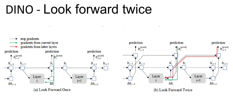
In DETR, a stop-gradient is applied between decoder layers to ensure stability, which forces each layer to optimize in isolation.

DINO allows the prediction results of the current layer to affect the parameter updates of the first two layers. This strategy enables the model to better utilize the gradient information of subsequent layers to optimize the parameters of early layers, thereby significantly improving detection accuracy

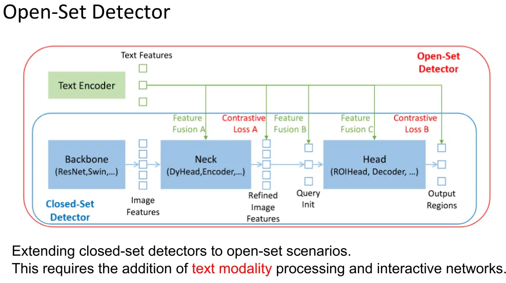
Grounding DINO

an open-set detector:

Changeable categories
Open scenarios
Zero-shot predict
Multimodal learning

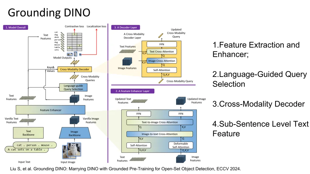
Deformable attention: only samples a small number of sparse key sampling points around each query, instead of attending to all positions, which greatly reduces computation and improves efficiency for vision tasks.
corss-attention

\boldsymbol{A} = \mathrm{Softmax}\left( \frac{\boldsymbol{T}\boldsymbol{I}^\top}{\sqrt{d}} \right)

\boldsymbol{O} = \boldsymbol{A} \cdot \boldsymbol{I}

LLM brief intro#

Tokenization & BPE#

Word tokenization
- Word tokenizers require lots of specialized rules about how to handle specific inputs
- With word level tokenization, we have no way of assigning an index to an unseen word! This means we don’t have a word embedding for that word and thus cannot process the input sequence
- $<UNK>$ lose lots of information about texts with a lot of rare words / entities
- Word-level tokenization treats different forms of the same word (e.g., “open”, “opened”, “opens”, “opening”, etc) as separate types -> separate embeddings for each
character tokenization

It greatly increases the length of input sequences, raising the computational overhead and sequence processing pressure for models such as the Transformer.
subword tokenization & Byte pair encoding
1. Form base vocabulary (all characters that occur in the training data)
2. count up the frequency of each character pair in the data, and choose the one that occurs most frequently
3. choose the most common pair (ug) and then merge the characters together into one symbol. Add this new symbol to the vocabulary. Then, retokenize the data
4. Keep repeating this process
5. Eventually, after a fixed number of merge steps, we stop
- to avoid $<UNK>$ , all possible characters / symbols need to be included in the base vocab. This can be a lot if including all unicode characters (there are ~138K unicode symbols)!
- GPT-2 uses bytes as the base vocabulary (size 256) and then applies BPE on top of this sequence (with some rules to prevent certain types of merges).
Limitations of subwords
- Hard to apply to languages with agglutinative (e.g., Turkish) or non-concatenative (e.g., Arabic) morphology
- Pretokenization rules don’t work on some languages (Thai, Chinese don’t use spaces between words; Hawaiian uses punctuation as consonants)

Transformer-Based Models#

Encoder-only transformer: BERT (full attention is used)
Decoder-only transformer: GPT, DALL-E, Robot control (only masked attention is used) downstream task

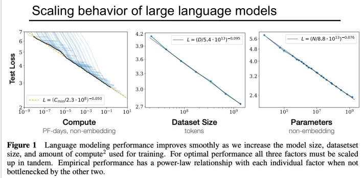
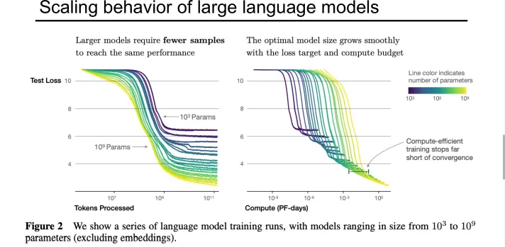
Scaling Laws#

Model performance is jointly determined by three factors: the number of parameters (N), training dataset size (D) and training compute (C), and follows a power-law relationship. All three factors must be scaled up simultaneously; increasing only a single dimension will lead to diminishing returns.

GPT-3#

if the model and training datasets are big enough, model can adapt to new tasks without fine-tuning

fewshot learning
One-shot learning
zeroshot learning

Alignmnet#

Alignment aligns LLM behavior with human values: SFT first establishes basic instruction-following, then RLHF builds on it to refine responses toward human preferences. this is not a part of this course, but it is quite important.

pretraining

SFT

RLHF

PPO
DPO
GRPO

Without SFT, RLHF has no foundation to build upon (the random policy’s exploration space is too vast); with SFT alone, the model’s upper bound is limited by the quality of the demonstration data.

prompt engineering#

CoT and so on

Parameter Efficient Fine-Tuning (PEFT)#

Few-shot Learning

Fine-Tuning vs. In-Context Learning

even for very large LMs, fine-tuning often beats in-context learning

In a fair comparison of fine-tuning (FT) and in-context learning (ICL), we find that FT outperforms ICL for most model sizes on RTE and MNLI

Parameter Efficient Fine-Tuning

Goal: perform fine-tuning of fewer parameters, but achieve performance on a downstream task that is comparable to fine-tuning of all parameters

Subset (top-k layer)

Pick a subset of the parameters and fine-tune only those (e.g. only the top K layers of a K+L layer deep neural network) 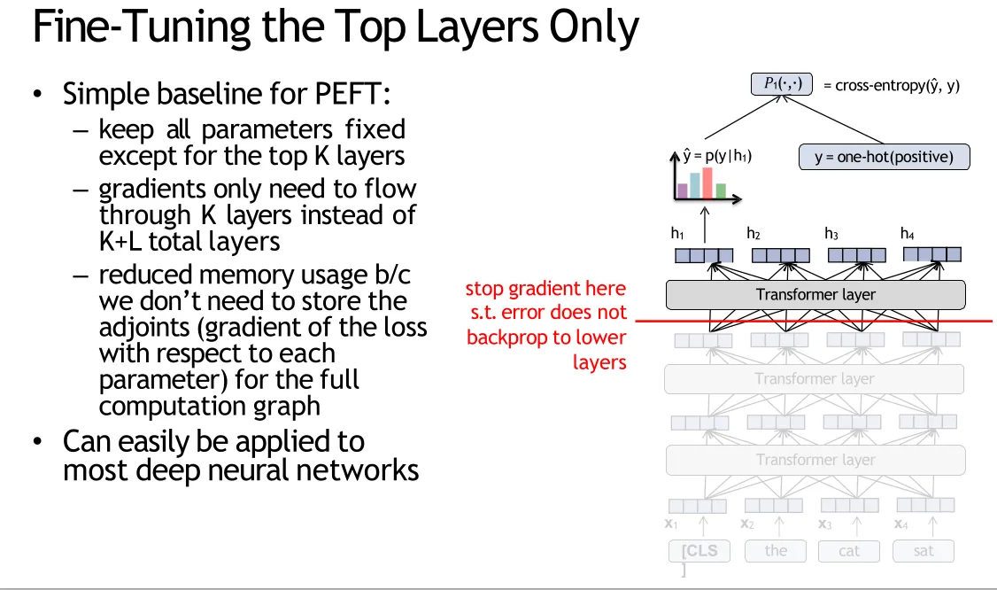The underlying network of the pre-trained LLM has already extracted general linguistic features (syntax, semantics, basic representations). Downstream tasks only require task-specific feature mapping and classification on top of these general features. Fine-tuning only the top layers is sufficient to accomplish the task, and the general features in the lower layers do not need to be modified.

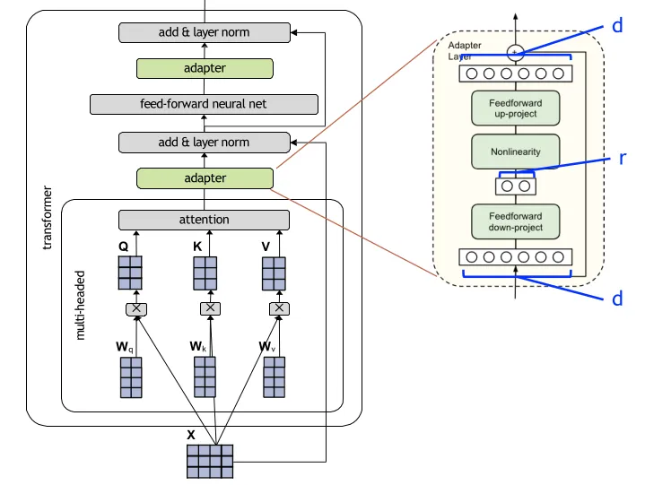
Adapters

add additional layers that have few parameters and tune only the parameters of those layers, keeping all others fixed

An adapter layer is simply a feed-forward neural network with one hidden layer, and a residual connection
For input dimension, d, the adapter layer also has output dimension d, but bottlenecks to a lower dimension m in the middle
Adapters achieve nearly the performance (i.e. 0% delta) of full fine-tuning but with substantially fewer parameters
Sometimes adapters even outperform full fine-tuning
MLM Pretraining

Rather than trying to predict the next word from the previous ones mask out a word (or a few words) and predict the missing words from the remaining ones

The main disadvantage of Adapter is that it introduces additional inference latency and parameters: because extra computation modules are inserted into the middle of the model, even if each module is small, they add computational time and memory access overhead during inference; additionally, each task requires saving its own set of Adapter parameters, so resource consumption accumulates when deploying multiple tasks.

Prefix Tuning

for a Transformer LM, pretend as if there exist many tokens that came before your sequence and tune the keys/values corresponding to those tokens 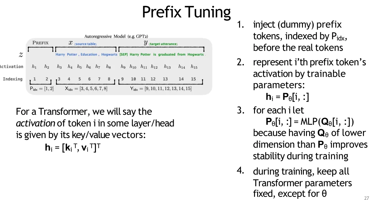Also works for encoder-only Transformer models, but we inject prefix tokens before both the source tokens x and the target tokens y

this is not in prompt. For the same downstream task, the prefix is fixed after training is completed.

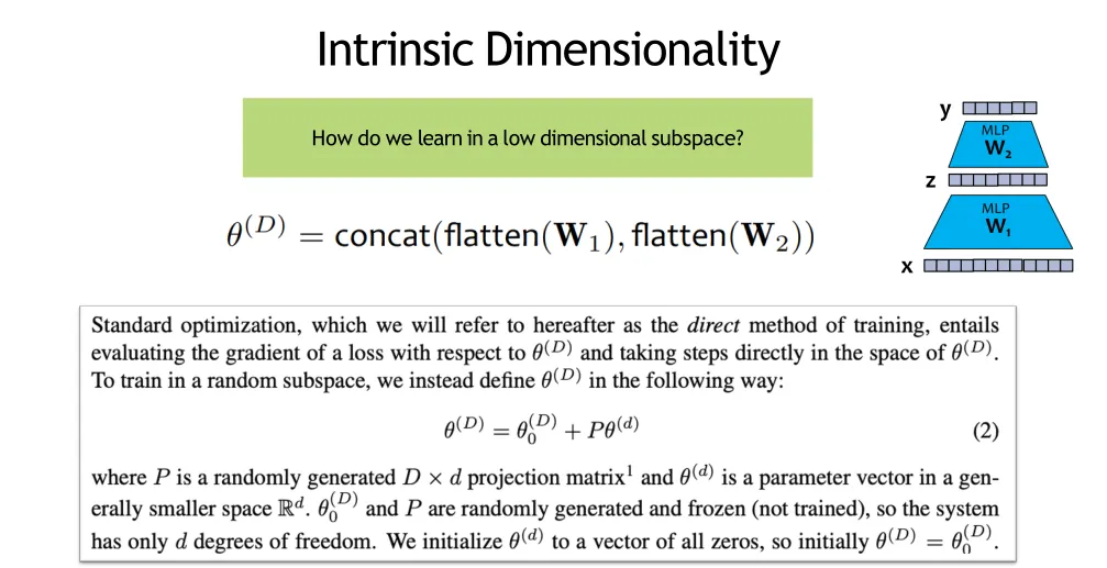
Intrinsic Dimensionality

the number of parameters in a model is not a great measure of how many degrees of freedom are needed to successfully learn some problem (maybe it is too much)

Intrinsic Dimension Definition from Li et al. (2018):

Learn a neural network with D parameters in a random lower dimensional subspace, d
Then repeat, gradually increasing the dimensionality, d
Let the intrinsic dimension be the value of d when good solutions (above 90% threshold of full parameterization) start to appear

Empirical results suggest that pre-training finds parameters that have low intrinsic dimensionality Aghajanyan et al. (2020)

LoRA

learn a small delta for the each of the parameter matrices with the delta chosen to be low rank

Motivation 1: “We take inspiration from Li et al. (2018a); Aghajanyan et al. (2020) which show that the learned over-parametrized models in fact reside on a low intrinsic dimension.”
Motivation 2: Directly optimizing the prompt, as in prefix tuning, leads to non-monotonic changes in performance as the number of parameters increases (we want more parameters to mean better performance!)
Motivation 3: Adapters and related methods introduce inference latency at test time that is non-trivial!

Key Idea

Keep the original pretrained parameters W0 fixed during fine-tuning
Learn an additive modification to those parameters $ΔW$
Define $ΔW$ via a low rank decomposition: $\Delta W = BA$ where BA has rank r, which is much less than the input dimension k or the output dimension d

Initialize

$A_{ij} \sim \mathcal{N}(\mathbf{0}, \mathbf{\sigma^2}), \forall i,j \text{ and } B = 0$
This ensures at the start of fine tuning, the parameters have their pretrained values: $\Delta W = BA = 0 \text{ and } W_0+BA = W_0$

Hot Swapping Parameters $W_0$ and BA have the same dimension, so we can ”swap” the LoRA parameters in and out of a Standard Linear Layer where $r << min(d, k)$

Takeaways

Applied to GPT-3, LoRA achieves performance almost as good as full fine- tuning, but with far fewer parameters
On some tasks it even outperforms full fine- tuning
For some datasets a rank of r=1 is sufficient
LoRA performs well when the dataset is large or small

PEFT FOR VISION TRANSFORMER

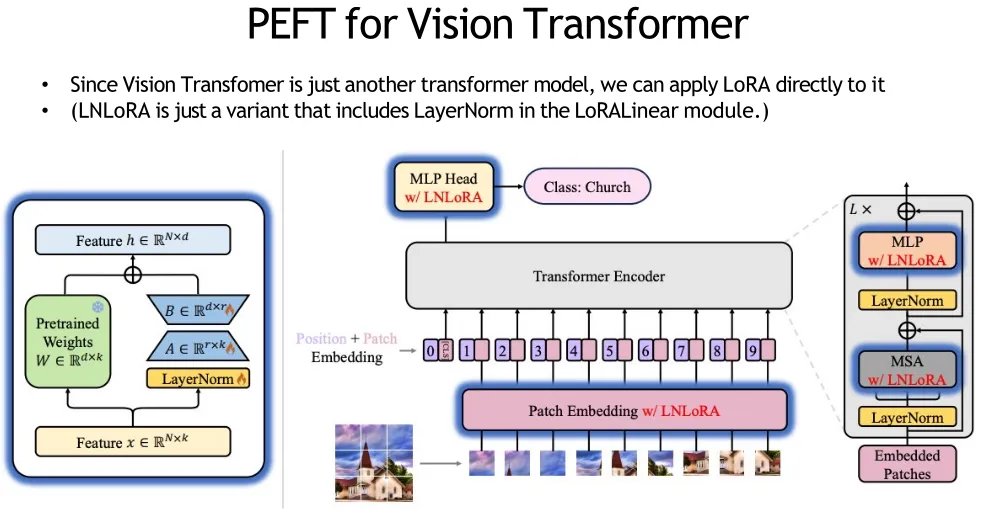For various computer vision tasks, parameter efficient transfer-learning (PETL) is sometimes better than full fine-tuning!